Chapter 8 General discussion

Part I: Forms of MELD

In Chapter 2, we showed that hyponatremia increased 90-day waiting list mortality. We also found that MELD-Na was a significantly better predictor of waiting list survival than MELD. Prioritization based on MELD-Na survival predictions could therefore reduce waiting list mortality. However, in the Eurotransplant region, MELD-Na is still not used for liver allocation.

Sodium levels and post-transplant survival

One of the concerns in the Eurotransplant community was that prioritizing hyponatremic patients for LT could decrease post-transplant survival. This concern arose in part because pre-transplant sodium levels are associated with increased morbidity, complications, and hospital admission.¹ Some older European studies indeed showed decreased short-term post-transplant survival in hyponatremic LT recipients.^2,3 Still, in recent Eurotransplant data, we found no significant post-transplant survival differences between normo- and hyponatremic LT recipients (data not published). This is in agreement with the largest study on post-transplant sodium effects in the US.⁴ MELD-Na evaluation also showed that after implementing the score for allocation, the negative effect of hyponatremia on waiting list mortality was greatly reduced.⁵

In the US, MELD-Na was implemented for MELD>11 patients after studying the effect of serum sodium levels on both survival with and without LT.⁶ Ideally, such analyses would also have been done in Eurotransplant. However, the required longitudinal sodium data is not available, as sodium is not adequately registered. In our validation study, we had to exclude two-thirds of eligible patients at baseline due to missing sodium. This missingness forms the most important limitation and rationale of our MELD-Na validation study. MELD-Na implementation could further improve waiting list ranking than found in this study because missing data analysis suggested that hyponatremia likely was more prevalent in patients with missing sodium data, as these patients significantly more often had alcohol-induced cirrhosis and higher creatinine levels. The seminal validation study of MELD by Wiesner et al. also excluded 48% (n=3,214) of patients due to missing data.⁷ This illustrates that sometimes evidence of improvement is provided despite missing data.

Sodium levels and renal function

Another concern was that increasing priority based on serum sodium levels would increase LT access for patients with renal dysfunction. Liver cirrhosis leads to portal hypertension and pooling of blood in the splanchnic bed. This lowers effective circulating blood volume, which increases the risk of renal dysfunction and renal failure.⁸ Hyponatremia in cirrhosis results from the renal compensation of the lowered effective circulating blood volume due to vasodilatation.¹ Considering lowered serum sodium levels could therefore increase waiting list priority and transplantation rates for patients with renal dysfunction over patients with liver failure alone.

However, (over)prioritization of patients with renal dysfunction is more likely caused by the high relative weight of creatinine in MELD than by the incorporation of serum sodium. MELD was developed in a cohort wherein patients with renal failure were excluded.⁹ In these patients, high creatinine levels likely indicated hepatorenal syndrome (HRS). Treating HRS with LT can reverse renal dysfunction postoperatively. Therefore, creatinine received a high weight in MELD, i.e., an increase in creatinine levels greatly increases MELD scores and transplant access. After construction, subsequent MELD validations were done in LT waiting list populations where patients with renal dysfunction were included.^7,10 This resulted in increased prioritization and transplantation for all patients with renal dysfunction,^11,12 whereas the aim of creatinine’s weight in MELD was to increase transplant rates for patients with HRS.

Interestingly, after MELD’s implementation, the number of liver-kidney transplant candidates tripled.¹² Therefore, the concern of (over)prioritizing patients with renal dysfunction for LT is relevant, but argues mostly against the current form of MELD. For the Eurotransplant region, a possible clinical solution could be to optimize patient’s renal function before transplantation. This would however also lower a patient’s ranking on the waiting list. Perhaps a better statistical solution could be to reweigh MELD’s parameters to decrease the importance of creatinine in LT allocation priority. It must be kept in mind that measuring creatinine and estimating GFR tends to overestimate renal function in cirrhotic patients,^13,14 creatinine is however widely available.

The Eurotransplant region uses a form of MELD that was constructed 20 years ago in 231 US patients. In its current form, MELD therefore does not represent the Eurotransplant population. Moreover, the predictive power of MELD is decreasing, as shown in Chapter 2 and in literature.¹⁵ In Chapter 3, we aimed to investigate whether updating MELD’s coefficients and bounds for the current Eurotransplant population would improve survival prediction for patients on the waiting list. We found that the refit models indeed significantly outperformed older non-Eurotransplant forms of MELD.

Beyond linearity

Refitted MELD and MELD-Na were based on the best fit in recent data to establish new parameter coefficients between new bounds. Refit MELD(-Na) is a linear model and splits continuous data into evidence-based categories, e.g., the proposed creatinine bounds of 0.7 and 2.5 mg/dL. The advantage of linear parameter relations to mortality is easy interpretation and computation. Some disadvantages are discussed below.

First, information was lost, as we forced linearity where the data showed non-linear parameter relations to mortality (e.g., sodium level relation to 90-day mortality). By categorizing continuous parameters, we assumed relations to be constant within each category but different between categories, which is not true. For example, we assumed that an 0.1-point creatinine increase from 0.7 to 0.8 mg/dL and from 2.4 to 2.5 mg/dL would give the same increase in risk of mortality. Then, for an increase from 2.5 to 2.6 mg/dL, a very different (constant) relation was assumed. This clearly is suboptimal. Still, these new bounds and resulting coefficients were a significantly better fit than those of UNOS-MELD. This implies that capturing the majority of patients with the right coefficient is most important.

Second, parameter lower and upper limits were set for the linear models. Beyond these limits, linearity broke down and parameter values were kept constant. Still, many patients had values beyond these limits. For example, 55% of Eurotransplant patients had a creatinine level below 1 mg/dL at listing, which was set to 1. Capping lower creatinine values might especially disadvantage female LT candidates, as measured creatinine overestimates their renal function,¹⁶ which results in MELD underestimation of mortality and perhaps unequal transplant access. To counter this inequality, additional MELD points for women have been suggested.¹⁷ Another possibility would be to express renal function through estimated glomerular filtration rate,¹⁸ which is still based on creatinine. At the higher end of creatinine levels, a limit was set to 4 mg/dL, again without evidence based on mortality risks.¹⁹ This upper limit also served to decrease the LT access for patients on dialysis, as all dialysis-dependent patients were set to this value. We proposed a new evidence-based upper limit for creatinine. Additionally, the need for dialysis could be incorporated in MELD as predictor, interacting with creatinine levels.

We especially argue against MELD’s lower limits of 1 for creatinine, bilirubin, and INR, as these were chosen to prevent negative MELD scores after log-transforming values below 1.¹⁹ Furthermore, we believe that survival probabilities should be used instead of MELD scores. Firstly, because this would eliminate the abovementioned arbitrary lower bounds of 1. Secondly, although clinicians have become used to communicating 90-day survival probabilities through MELD scores, they are an unintuitive and unnecessary translational step from actual probabilities to arbitrary scores. Currently, a 50% chance of being alive after 90 days is communicated to patients and clinicians as a MELD score of 30, which is arguably less easily understood. Primarily communicating survival probabilities would benefit both patients and clinicians.

MELD 3.0

Recently, MELD 3.0 was proposed, which refits MELD-Na and adds serum albumin, patient sex, and significant interactions.²⁰ Interestingly, MELD 3.0 improves none of the abovementioned limitations. Although non-linearity was present for sodium and albumin levels, a linear model was used. Lower bounds of 1 were kept. Reality is not linear, yet MELD is. Therefore, as alternative, in Supplement Chapter 10.1 we proposed to use a flexible, non-linear waiting list model.²¹ Such a spline-based model would capture non-linear relations and thus provide a better fit to the data. A concern could be that the model would overfit. However, this seems unlikely given the large data sample and small number of predictors. A model best represents the population it was constructed in. Parameter relations to mortality will change over time within the same population, which for MELD resulted in decreased prediction performance.^15,22 The established model can be a bad fit to other independent datasets, which we confirmed by refitting the 20-year-old UNOS-MELD in a recent Eurotransplant dataset. This is why regular updates of prediction models are recommended.²³ The fear of overfitting therefore should not prevent updates that bring valuable improvements for patients on the waiting list.^15,24

Part II: Disease over time

MELD’s linearity reduces non-linear reality. MELD 6-to-40 scores are used instead of survival probabilities. Longitudinal data is registered but is currently ignored. Current prediction models are static but should be dynamically updated based on newly available data. Using MELD at one single moment does not acknowledge changes over time and how these changes are related to survival. Clinicians intuitively update estimates of patient life-expectancy with changing patient condition and measurements.

These formed the reasons to investigate LT candidate survival prediction models that could meet these demands. In Part II of this thesis, we aimed to better approximate a clinician who evaluates patient prognosis.

Approximation of disease severity over time

Current waiting list survival predictions are based on measurements at one moment in time, i.e., the last measurement available. However, previous data provide important information about the severity of disease and its rate of change over time.^25,26 The second part of this thesis therefore focuses on joint models (JMs), which combine longitudinal and survival analysis. This allowed investigation of the effect of changing MELD scores over time on patient survival.

Previously, time-dependent Cox (TDC) models have been used to model MELD scores and waiting list survival over time.^25–31 In TDC analysis, the changing temporal effect of a predictor is estimated based on follow-up time divided into intervals of measurement, e.g., 0-30 days and 31-60 days. Within each time interval, TDC models assume that the last measured value is carried on forward. In the abovementioned example, creatinine values measured on day 0 and 31 would remain constant for the next 30 days. Crucially, there is no interpolation of values, thus a creatinine value at e.g. day 45 is not approximated.³² In clinical terms, the TDC assumes that the disease state does not change until the next moment of measurement. This results in a ‘staircase effect’, where the trajectory of disease over time is represented through rectangular steps, see Figure 8.1. Survival is then predicted based on this staircase trajectory.

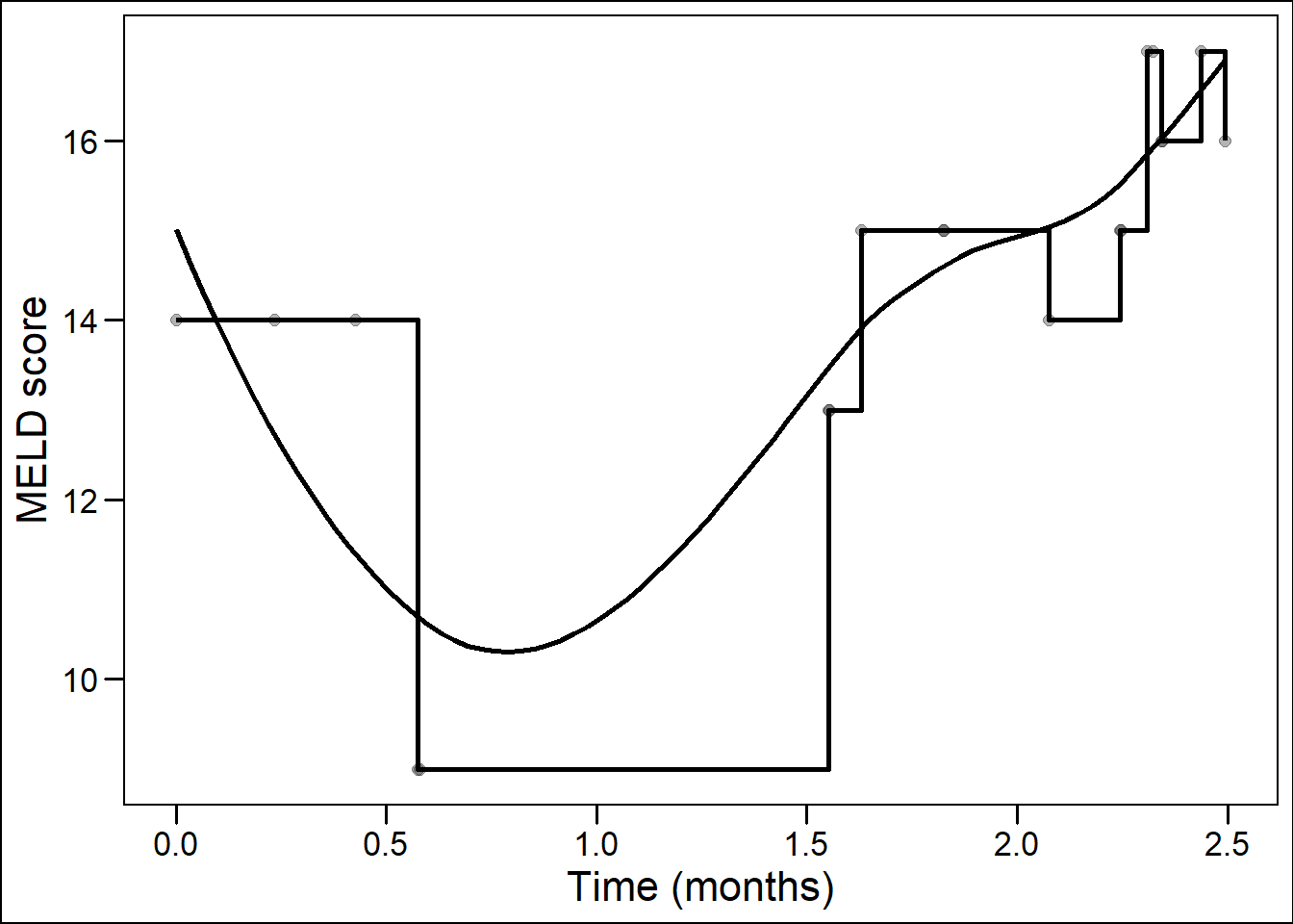
Figure 8.1: Staircase versus smooth representation of disease over time.

However, it is clinically evident that the condition of a patient and the liver disease are not constant until a new moment of measurement. Instead, disease develops continuously, as a smooth and non-linear trajectory. We configured JMs to estimate disease as a smooth continuum over time with interpolation of trajectories between measurements. At and between measurements, not the last measured value was assumed, but the ‘true’ underlying value. For the abovementioned example, the JM would estimate values for each moment in time between day 0 and 60. Crucially, the model considered that measurements from the same patient were more related than measurements between patients. TDC models ignore this correlation.

Another advantage of extrapolating the true underlying trajectory is that missing values are filled in. Missing values therefore have less effect on estimated survival. We therefore believe that JMs are better suited for real-life cohort data, where disease is continuously developing and where measurements are correlated and can be missing. The performance of JMs versus TDC models was previously assessed in small and theoretical simulation studies, where JMs showed significantly improved performance over TDC models.^33–35 However, JMs were never applied to large cohorts of patients nor to the field of LT. In Chapter 4, Chapter 5 and supplement Chapter 10.2, we therefore investigated JMs as alternatives for survival prediction in LT candidates.

Joint modeling disease and survival over time

In Chapter 4, we fitted JMs to waiting list data of the Eurotransplant and UNOS regions. The JMs modeled average and individual MELD scores and considered both the value of MELD(-Na) and its rate of change at each moment in time. For the first time, liver disease was considered as developing entity within each patient on the waiting list.

Underlying MELD value

The observed, that is measured, values of MELD(-Na) scores have been used in liver graft allocation for 20 years. The JM uses these observed measurements to estimate the ‘true’ underlying disease trajectory. The model can therefore assume a different MELD(-Na) score than is observed for each patient. For example, for actively listed LT candidates in the Eurotransplant region between 2007-2018, the median measured value of MELD at the start of listing was 15 ( Table 4.1 ). However, the JM assumed a baseline MELD value of 17.8, which is notably higher. In addition, for each patient, the JM considered the individual deviation from the average MELD(-Na) score at a given moment in time. This placed patients in context to the population average. The individual deviations from the average were also used as prognostic information in survival prediction. Naturally, the question arose whether this underlying disease severity should be used over actually measured disease.

Prediction performance based on underlying trajectories

Interestingly, when predicting waiting list survival, the JM outperformed MELD both at baseline and during follow-up. This implied that 1) the JM-estimated underlying disease severity better corresponded with survival than observed MELD values and 2) using individual deviation from the population average added prognostic information. The estimated underlying disease trajectory is less sensitive to missingness or errors. JMs can however be severely biased if they are mis-specified, particularly in the specification of longitudinal trajectories.³³ Therefore, we considered multiple configurations of spline-based and linear mixed effect models (longitudinal part of the JMs) and assessed their fit through Akaike information criterion (AIC) values. Most notably, the use of spline-based instead of linear-approximated patient trajectories greatly improved model fit.

Over time more waiting list data per patient typically becomes available. Therefore, after listing, the JM predictions became increasingly accurate within each patient as follow-up increased, which contrasts to MELD(-Na). Little attention is given in literature to the fact that MELD is a Cox model constructed and validated to first listing data.^7,9,10 However, most patients on the waiting list are months away from first listing. When assessing JM and MELD performance over time, a decline in discrimination and accuracy was shown. The patients who survived longest on the waiting list despite their MELD scores likely had a better condition beyond what MELD measured, or vice versa. However, since only MELD was measured, over time it became more difficult to predict survival in the resulting population. Still, JM performance was significantly better than MELD performance for most follow-up times. Also, in our analysis, all patients started from the same moment in time (first listing). However, on the actual waiting list, patients are constantly added and removed. In other words, survival prediction for liver graft allocation is based on cross-sections, not a cohort. In real waiting list data, MELD’s discrimination is therefore likely to be lower, as the sickest patients are transplanted quickly and ranking the remaining less ill patients is more difficult. The JM accuracy increases with more available measurements over time. Because of this, we would not expect a similar decrease in performance if the JM would be applied to the actual waiting list.

Joint modeling acute-on-chronic liver failure

ACLF and MELD-Na

Liver disease is constantly changing. In clinical practice, the rate at which a patient changes directly influences medical urgency and possible intervention. This might be especially true for patients with acute-on-chronic liver failure (ACLF). ACLF is characterized by initially stable and chronic liver disease, which rapidly deteriorates after a predisposing event and leads to multi-organ failure and often death.³⁶ Timely transplantation can save a subset of these patients,³⁷ but MELD-Na underestimates ACLF mortality and therefore the need for transplantation.^38,39

In supplement chapter 10.2, we hypothesized that JMs would be suited for predicting ACLF survival.⁴⁰ First, because each individual patient’s condition can change rapidly. Therefore, it is relevant to predict survival based on both past and current data. It is also relevant to place the individual disease and survival in context to the population average. Second, by using both measured disease severity and its rate of change over time, the acceleration in ACLF severity is linked to future survival. Third, updating future predictions at each new measurement is relevant in patients with increasing disease severity.

In Chapter 5, we approximated liver disease severity in ACLF patients based on repeated MELD-Na values, corrected for baseline ACLF grade and other predictors (sex, age, presence of cirrhosis, life-support dependency, and presence of bacterial peritonitis). However, predicting ACLF survival based on MELD-Na measurements was suboptimal. This is because ACLF involves inflammation and multi-organ failure,³⁶ which are not captured by MELD-Na scores. Therefore, ACLF survival prediction could be improved further by modeling more organ system functions over time. Survival prediction based on simultaneous consideration of multiple organ systems is possible in multivariate JMs. It would make sense to separately consider the role of each organ system. Unfortunately, such data is not readily available for both the Eurotransplant and UNOS regions. Therefore, like others,^37,38,41 we could only correct for ACLF grade at baseline. However, within the European Foundation for the study of Chronic Liver Failure (EF CLIF) consortium data, longitudinal CLIF ACLF scores measurements per patients could be available. Therefore, future application of JMs in this data might result in JMs that better represent changes in ACLF and let failure of each organ system correlate to mortality.

Underlying MELD rate of change

Despite using MELD-Na as basis, we still hypothesized that improvement was possible, mainly because baseline ACLF severity and MELD-Na rate of change would be considered. For the rate of change, the term ‘slope’ is often used, as the rate of change is the derivative of the function of MELD-Na values over time. The concept of MELD-Na’s rate of change (or slope) over time is not new. Most notably, delta-MELD has been proposed previously.²⁵ However, the slope generated by the JM differs notably from delta-MELD. Firstly, the JM slope is based on the assumed true underlying disease development (see above). Secondly, the JM slope is the derivative of the measured value at one specific moment in time. In contrast, delta-MELD is defined as the difference between the current MELD score and the lowest MELD score in the previous 30 days, divided by the number of days between the current and lowest scores.²⁵ Thus, the obtained delta-MELD slopes are averaged over a varying number of days for different patients and time points. Also, using the lowest previously measured value overestimates the rate of change, unless the previous value actually is the lowest. This way, delta-MELD could indicate increasing disease severity even though a patient was in stable condition, see Figure 8.2. Basing treatment decisions on such estimates therefore seems inappropriate. In the example below, the JM slope would be approximately horizontal at 30 days and therefore the instantaneous slope at each moment is a better representation changing disease.

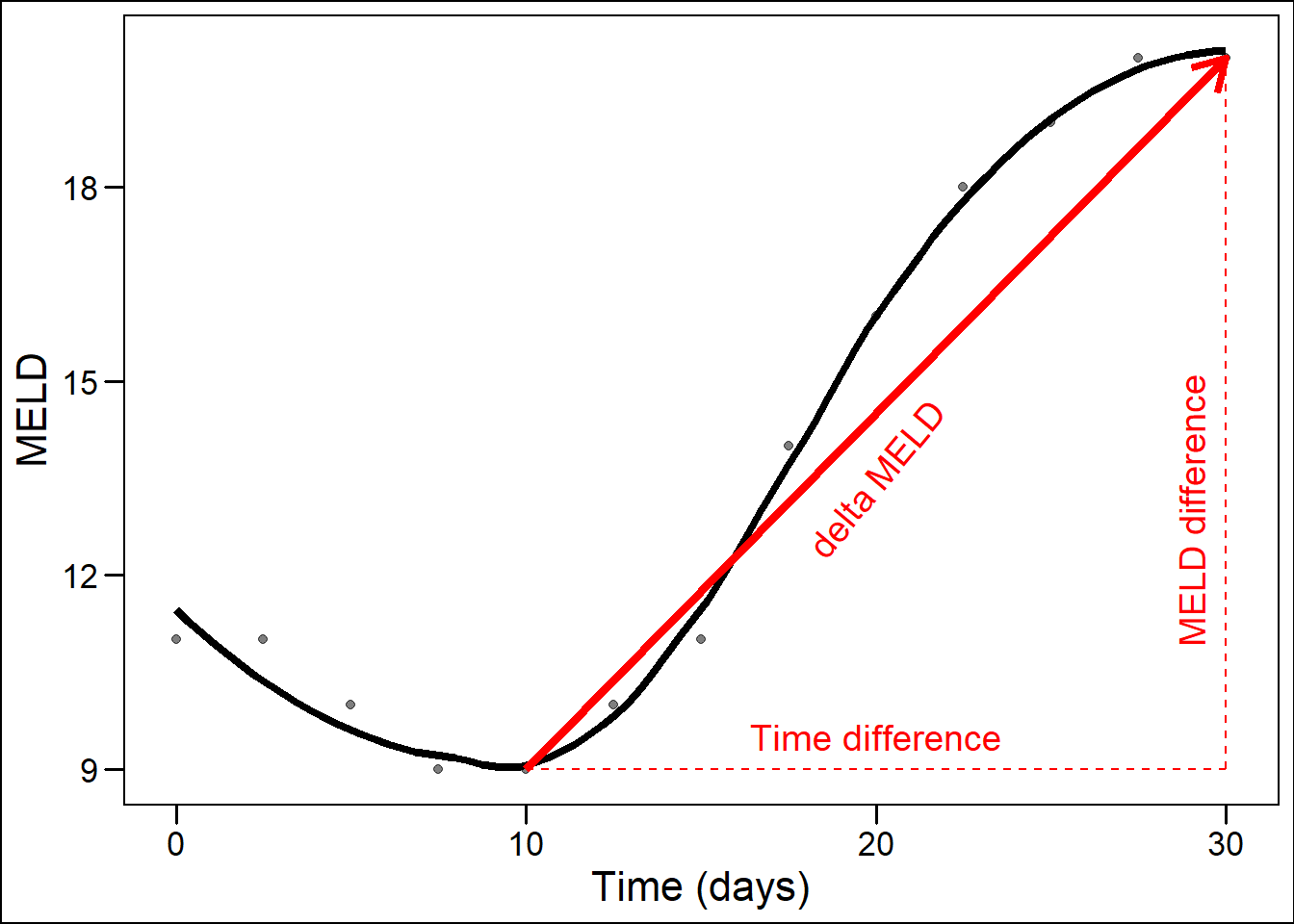
Figure 8.2: Illustration of delta-MELD slope overestimation of disease increase.

Lastly, the effect of delta-MELD on waiting list mortality depends on the number of previous MELD measurements.⁴² This causes bias for survival prediction on the LT waiting list, as the severity of disease determines the number of measurements. For example, a clinician could increase the frequency of measurement after a patient’s disease worsens, or vice versa. Thus, measuring MELD and delta-MELD in sick patients corresponds with death, but an improvement would likely be less easily observed. Therefore, Delta-MELD depends on the number of measurements, which causes bias that will increase its apparent usefulness.²⁶ Despite this bias, the concept of delta-MELD is used often.^5,28,43–48 In our view, this stipulates the need to adequately incorporate MELD’s rate of change in survival prediction. The JM is not biased by the number of measurements, as it estimates a continuous underlying trajectory. Still, with increasing measurements available, the trajectory of the patient will be more accurately reflected.

Personalized predictions

Because JMs consider both the average and individual development of disease, survival predictions can be personalized. Consider that a Cox model uses coefficients, derived from a studied population, to predict outcome. These coefficients can be viewed as the average parameter-mortality relationships of a studied population. However, applying these coefficients on an individual level will give only an average prediction of survival. A patient could ask her physician: “ How long will I survive with my current disease?” Based on a MELD score, e.g. 20, the physician could give a prognosis estimate based on population averages counted from baseline. In other words, a correct answer would be: “ If there would be 100 patients with your MELD score 20, we estimate that on average 10% will have died within three months after first waiting list registration.” After this clarification, questions and uncertainty remain for the patient and possibly also for the physician, because of several reasons.

First, the patient does not know how ‘average’ she is, that is how well the average parameter-mortality relation will apply to her. This is why considering individual patient trajectories through joint-modeling is valuable. Second, the patient is most likely not at the moment of first registration but beyond that, at some later point in time, which is why it is better to use accumulating data over time and update predictions accordingly. Third, clinicians could also miss that MELD’s predictions were only validated on baseline populations.^7,9,10

We believe that the personalized predictions can benefit both the patient and the clinician. The main reason being that the patient is recognized as unique entity and is not abstracted into population averages. The clinician can also be more confident that the predicted prognosis applies to the individual patient. Therefore, personalized JM predictions were made available at https://predictionmodels.shinyapps.io/meld-jm/.

Part III: Survival with and without transplantation

Benefit from liver transplantation

The final part of this thesis studies a simple question: “does transplantation improve survival?” In Chapter 6, we investigated whether LT caused survival improvement for patients on the waiting list. The difficulty is that such causal effects, that is the difference between transplanting and not transplanting, cannot be observed, as each patient is either transplanted or not. It would be considered unethical to conduct a randomized trial on LT survival benefit. Therefore, counterfactual waiting list survival of transplanted patients was estimated through inverse probability of censoring weighting (IPCW) analysis.⁴⁹ Benefit scores were calculated as the difference between survival with and without LT.

We used sequential stratification and IPCW to predict counterfactual waiting list survival, which is the waiting list survival of a transplanted patient if LT would not have been done. We applied these techniques because patients on the waiting list are transplanted after baseline and the donor graft is allocated depending on the severity of disease. See Figure 8.3 below, where four hypothetical patients on the waiting list are shown (three severely ill, one less ill). In this example, patient 2 is dependently censored at transplantation and therefore survival of remaining and comparable patients is given more weight. Each patient was listed at a different point in time (t0) and therefore spent a variable amount of time waiting at the cross-section. Survival is counted from the moment of cross-section and all patients receive equal weights (w=1). Due to high disease severity, patient 1 died before a liver graft became available. Patient 2 survived long enough and was transplanted. After transplantation of patient 2, patient 3 received more weight (w=2) to compensate for the missing survival time of patient 2 after censoring. Patient 4 (medium MELD) did not receive higher weight as its condition was not comparable to patient 2.

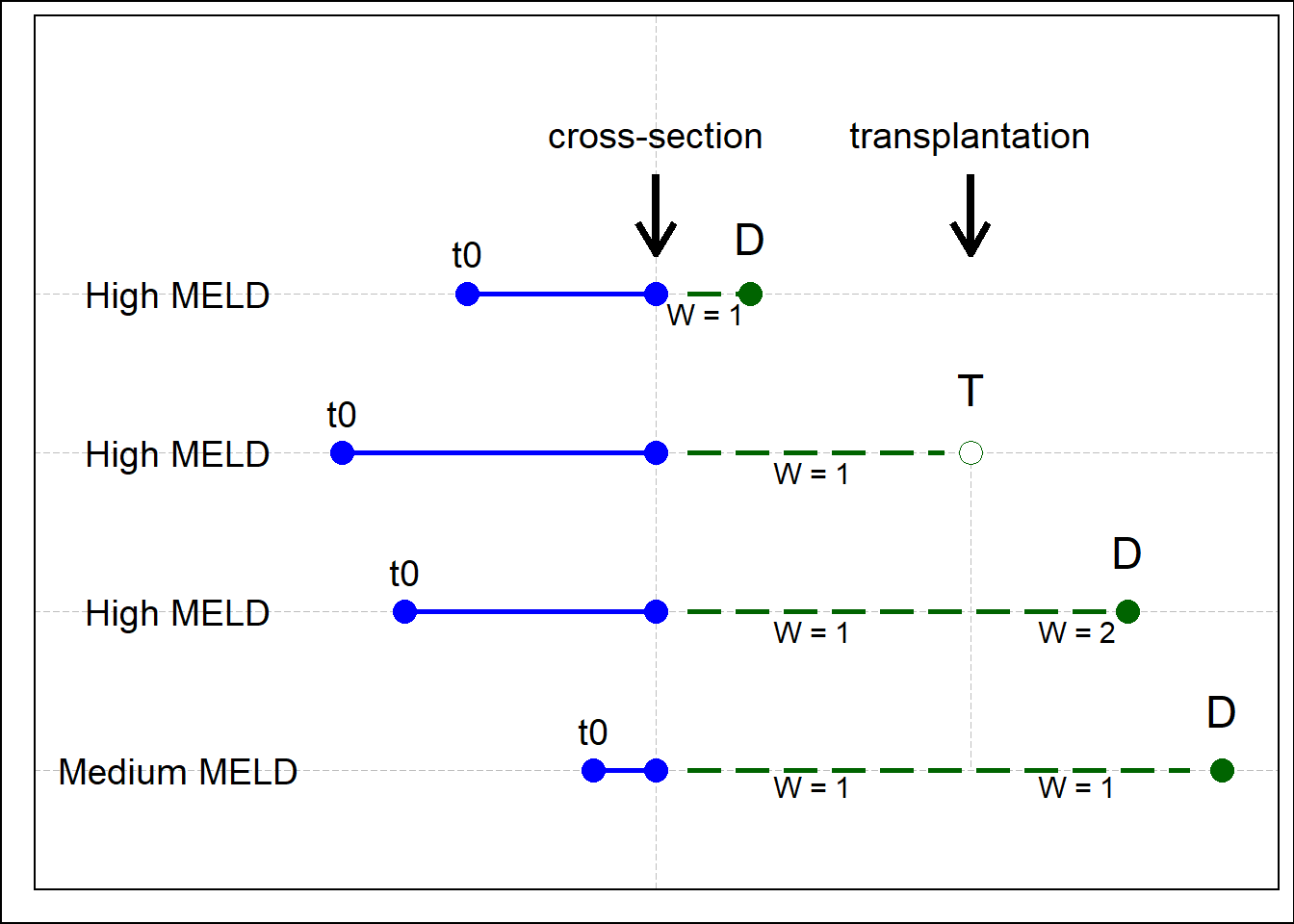
Figure 8.3: An illustration of IPCW. Note the change from w=1 to w=2 for patient 3. D: death, T: transplantation.

Validity

In the literature, benefit is often defined as the difference between post-transplant survival and waiting list survival counted from baseline.^50–54 The idea is to match patients with a similar disease state (e.g., MELD score) either at waiting list registration or transplantation. However, this definition of benefit assumes that two different patients at two different moments in time will yield survival curves that can be compared. We argue against these assumptions. Firstly, the fact that two patients have the same MELD score, perhaps with some more similarities like age and sex, does not make their state of disease comparable. We showed this to be true in Part II, where we showed that 1) previous disease development is different between two persons and 2) the rate of change in disease severity significantly influences future survival. This is perhaps best illustrated in Figure 4.1. Secondly, following from the previous arguments and the fact that liver disease typically progresses over time, survival predictions based on two different moments in time should not be compared to estimate benefit. Third argument is that the decision to transplant or not is made at the moment of liver graft offering, not baseline. Fourth, the fact that MELD and other predictors can be measured at baseline or at transplantation does not mean that it is right to use only these, which is the law of the instrument.⁵⁵ Therefore, by comparing survival within patients based on previous disease and slope, we provided a more precise and valid definition of patient disease. Still, the validity of the time-dependent Cox benefit estimates could have been improved further by using JMs to better define disease severity.

Reliability

The reliability of benefit estimates was also improved. Firstly, because we estimated survival from a certain calendar moment in time (cross-section). This is important, as liver grafts are offered to cross-sections of patients, where each patient has previously waited a variable amount of time and survival is predicted from that moment on. Counting survival from baseline instead makes all patients start from the same moment in time. Secondly, we used weighting to 1) correct waiting list survival for dependent censoring bias and 2) estimate waiting list survival as if LT was not available as treatment. Careful consideration of which question is answered by which statistical method is important when estimating benefit.⁵⁶ In clinical terms: an example is making a distinction between the survival before LT and survival without LT, which are very different (Figure 6.1 ).

Careful consideration argues against using competing risks (CR) analyses to approximate waiting list survival without LT.^50–52 CR analysis estimates survival before LT and should be used to evaluate waiting list outcomes: transplantation, death, or removal.⁵⁶ It would be wrong to base allocation on CR-predicted future waiting list survival. To illustrate, consider a patient with MELD 40 (very ill) and a patient with MELD 20 (reasonably ill). A physician might predict correctly that the MELD 40 patient has a (much) higher chance of receiving a LT the next 90 days than the MELD 20 patient, as transplant chances increase with disease severity. In CR reasoning, we would then argue that the risk of death for the MELD 40 patient is lowered, as transplantation competes with death. However, it would be perverse to decrease allocation priority based on this reasoning, as the high chance of transplantation for the MELD 40 patient is a result of the high risk of death. Instead, priority should be based on the risk of death without LT,^49,56 which we properly modeled using censorship with adjustment for dependent censoring.

By correctly modeling waiting list survival without LT in the last part of this thesis, we must acknowledge, due to progressive insight, that the reliability of the previous survival prediction models in Part I and II could have been improved further. We modeled survival in a censorship framework but did not adjust dependent censoring bias through IPCW. This should have been done, as the priority for LT depends on MELD and the Cox model assumes that censored patients have the same chance of dying as patients who remain on the waiting list, which is not the case for transplanted patients. Since transplantation chances increase with MELD, the sickest patients typically spend the least time on the waiting list, because they are transplanted (and censored) more frequently and faster. Through IPCW, after a (high MELD) patient is transplanted, more weight is given to the remaining and comparable (high MELD) patients, who can survive some more time on the waiting list. Censoring without weights, which MELD(-Na) does, therefore leads to an increasing underestimation of mortality for patients with increasing disease severity, as death is more frequently prevented through transplantation (and after censoring outcomes and survival times are unknown). In other words, by using the unweighted MELD(-Na), current liver allocation is biased where it matters most, as it underestimates mortality in the sickest patients.

Logical continuation

Although the clinical relevance of causal models is evident, a problem is that their prediction performance cannot be assessed (yet).⁵⁷ Consider for example calibration, where predicted and observed risks are compared. This comparison cannot be done, as counterfactual waiting list survival is not observed. We are however confident about the obtained estimates. Firstly, because simulation studies showed that the used methods are valid.^49,58 Secondly, the future waiting list survival estimates of transplanted patients are a logical continuation of observed and corrected waiting list survival. An illustrative analogous example from mathematics is analytic continuation, where the domain of a function is extended in the only way possible that is preserving certain requirements. Consider Figure 8.4A below, where the lines in the right half of the plot represent a certain function (Riemann Zeta function, source: https://www.3blue1brown.com/lessons/zeta). Only the right half is shown, as only this side can be defined by the function. The left half of the plot in Figure 8.4B shows the analytically continued right half, which is continued from the right based on requirements such as line angles. However, the left half cannot be defined by the function that plots the right half, even though its continuation is logical and can be visualized. This is analogous to estimating without LT survival (left half) based on observed waiting list survival (right half), which is a logical continuation based on available data, but by definition cannot be observed nor validated.

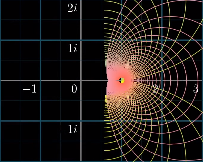
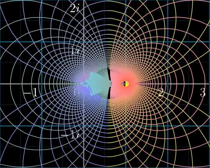
Figure 8.4: Analytic continuation of the Riemann zeta function.

Although causal models currently cannot be validated, benefit allocation policy has been based on these methods, most notably the MELD-Na implementation for patients with MELD>11 and UK benefit-based allocation.^6,30,59 We believe that the predicted survival without LT as possible treatment best serves as guide for transplantation assignment in future patients.^56,57,60

Further improvements of causal liver allocation models are possible. We performed a retrospective study of benefit. However, for prospective use in allocation, IPCW could be replaced by IPTW, that is inverse probability treatment weighting. IPTW differs from IPCW in that both survival with and without LT are estimated as future hypothetical risks, whereas in the IPCW analysis of Chapter 6 the with LT survival was retrospectively observed. IPTW further approximates clinical decision making based on expected outcomes with and without transplantation, as in reality both outcomes are hypothetical at the moment of liver graft offering. This requires clinicians to be comfortable with basing treatment decisions on hypothetical risks from models that cannot be validated (yet). However, this is what experienced clinicians do intuitively when evaluating an offered donor liver graft for a LT candidate. Indeed, the statistical machinery required to approximate clinical decision making is complex. This highlights the capabilities and intuition required from an experienced physician who is faced with the decision to transplant or not.

Two principles

We compared LT survival benefit of patients with and without HCC. This comparison is relevant because different allocation principles are applied to patients with and without HCC. The group of HCC patients is intended to be exemplary for other exception patients. With increasing HCC incidence,⁶¹ already inequal LT access might be worsened further.¹² For non-HCC patients, LT listing is based on expected waiting list survival, or the principle of urgency (sickest first). HCC patients are listed based on Milan criteria, which represent acceptable post-transplant survival.⁶² Considering post-transplant survival is the principle of utility, which ignores HCC waiting list survival and alternative pre-LT HCC treatment options.⁶³ Moreover, instead of patient characteristics, artificial exception points are used to express HCC waiting list priority, which further worsened the already inequal LT access between non-HCC and HCC patients.^50,64,65 Lastly, HCC patients within Milan criteria and within one region are prioritized on waiting time, which is inherently flawed, as waiting longest does not equal to highest waiting list mortality.^66,67 To resolve these issues, we proposed the use of survival benefit as single equalizing metric. Previous simulation showed that benefit-based allocation resulted in more life-years gained from the same number of available liver grafts.³⁰

However, if physicians and policy makers do not endorse benefit as metric, at least (non-)HCC waiting list survival should be estimated by a single pre-transplant survival model, which could be similar to our proposed weighted waiting list model. The use of actual patient characteristics to estimate both waiting list and post-transplant survival removes the need for the inherently flawed exception points. With the availability of HCC waiting list survival prediction models, there is no need for arbitrary and artificial inadequacy through exception points, as these are solely needed to compensate MELD(-Na)’s inability to predict waiting list survival in patients with preserved liver function. Policy and research should focus on collecting data and establishing models that adequately predict survival. This would remove the ongoing time-consuming arbitrary changes required for the exception point system. Survival prediction and liver graft allocation should be based on actual patient characteristics, not arbitrary points.